Learning PyTorch: Simple Linear Regression

Python

Author

Kai Tan

Published

April 20, 2024

In this post, I will demonstrate how to implement a simple linear regression model using PyTorch.

Data Generation

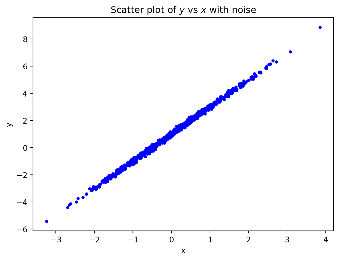
Generate $n = 1000$ data points from a linear model: $y_{i} = b_{0} + w_{0} * x_{i} + ε_{i}$

$b_{0} = 1$ and $w_{0} = 2$
$x_{i} \sim N (0, 1)$ and $ε_{i} \sim N (0, 0.01)$

import numpy as np
import matplotlib.pyplot as plt
rng = np.random.RandomState(42)
n = 1000
b0, w0 = 1, 2
x = rng.standard_normal(size=(n, 1))
e = 0.1 * rng.standard_normal(size=(n, 1))
y = b0 + x * w0 + e

print('true weight:', w0)
print('true bias:', b0)

plt.plot(x, y, 'b.')
plt.xlabel('x')
plt.ylabel('y')
plt.title(r'Scatter plot of $y$ vs $x$ with noise')
plt.show()

true weight: 2
true bias: 1

Solve Linear Regression by Gradient Descent in NumPy

Step 1: Given weight $w$ and bias $b$ , compute prediction (Forward pass): ${\hat{y}}_{i} = b + w x_{i}$
Step 2: compute the loss: $L (w, b) = \frac{1}{n} \sum_{i = 1}^{n} (y_{i} - {\hat{y}}_{i})^{2} = \frac{1}{n} \sum_{i = 1}^{n} (y_{i} - b - w * x_{i})^{2}$
Step 3: compute the gradients (backward pass): $\frac{\partial L}{\partial w} = - \frac{2}{n} \sum_{i = 1}^{n} (y_{i} - b - w x_{i}) x_{i} = - \frac{2}{n} \sum_{i = 1}^{n} (y_{i} - {\hat{y}}_{i}) x_{i}$ $\frac{\partial L}{\partial b} = - \frac{2}{n} \sum_{i = 1}^{n} (y_{i} - b - w x_{i}) = - \frac{2}{n} \sum_{i = 1}^{n} (y_{i} - {\hat{y}}_{i})$
Step 4: update the parameters: $w \leftarrow w - η \frac{\partial L}{\partial w}$ $b \leftarrow b - η \frac{\partial L}{\partial b}$

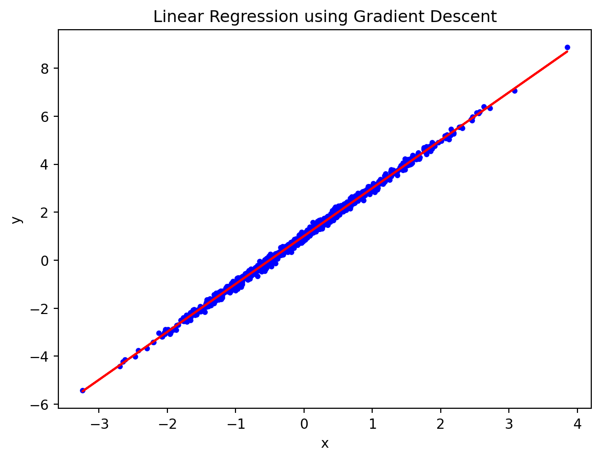
# initialization of weight and bias
w = rng.standard_normal(1)
b = rng.standard_normal(1)
print('Initial bias:', b)
print('Initial weight:', w)

lr = 0.01 # learning rate
n_epochs = 1000 # number of iterations
for t in range(n_epochs):
    # step 1: prediction
    y_pred = b + w * x
    # step 2: compute loss
    loss = np.mean((y - y_pred) ** 2)
    # step 3: compute gradients
    dw = -2 * np.mean(x * (y - y_pred))
    db = -2 * np.mean(y - y_pred)
    # step4: update weights and bias
    w -= lr * dw
    b -= lr * db
print('Final bias:', b)
print('Final weight:', w)

# plot the results
plt.plot(x, y, 'b.')
plt.plot(x, b + x * w, 'r-')
plt.xlabel('x')
plt.ylabel('y')
plt.title('Linear Regression using Gradient Descent')
plt.show()

Initial bias: [-0.14451867]
Initial weight: [-0.67517827]
Final bias: [1.00716318]
Final weight: [1.99588476]

Solve Linear Regression with PyTorch (autograd)

# using pytorch
import torch
import torch.optim as optim
import torch.nn as nn

torch.manual_seed(42)  # for reproducibility

device = torch.device('cuda' if torch.cuda.is_available() else 'cpu')
# convert data to torch tensors
x_tensor = torch.from_numpy(x).float().to(device)
y_tensor = torch.from_numpy(y).float().to(device)

lr = 0.1
n_epochs = 1000
# initial weights and bias
b = torch.randn(1, requires_grad=True, device=device)
w = torch.randn(1, requires_grad=True, device=device)

for t in range(n_epochs):
    # step 1: prediction
    y_hat = b + w * x_tensor
    # step 2: compute loss
    error = y_tensor - y_hat
    loss = torch.mean(error ** 2)
    # step 3: compute gradients (via autograd)
    loss.backward()
    # step 4: update weights and bias
    with torch.no_grad():
        b -= lr * b.grad
        w -= lr * w.grad
    b.grad.zero_()
    w.grad.zero_()
print('Final bias (PyTorch):', b)
print('Final weight (PyTorch):', w)

Final bias (PyTorch): tensor([1.0072], requires_grad=True)
Final weight (PyTorch): tensor([1.9959], requires_grad=True)

Solve Linear Regression with PyTorch (autograd + loss + optimizer)

b = torch.randn(1, requires_grad=True, dtype=torch.float, device=device)
w = torch.randn(1, requires_grad=True, dtype=torch.float, device=device)

lr = 0.01
n_epochs = 1000
loss_fn = nn.MSELoss(reduction='mean')
optimizer = optim.SGD([b, w], lr=lr)
for t in range(n_epochs):
    # step 1: prediction
    y_hat = b + w * x_tensor
    # step 2: compute loss
    loss = loss_fn(y_tensor, y_hat)    
    # step 3: clear old and compute current gradients
    optimizer.zero_grad() # clear old gradients
    loss.backward()       # compute current gradients
    # step 4: update weights and bias using the specified optimizer (e.g. SGD)
    optimizer.step()
    
print('Final bias (PyTorch with optim):', b)
print('Final weight (PyTorch with optim):', w)

Final bias (PyTorch with optim): tensor([1.0072], requires_grad=True)
Final weight (PyTorch with optim): tensor([1.9959], requires_grad=True)

Object-oriented programming

import torch
import torch.nn as nn

device = torch.device("cuda" if torch.cuda.is_available() else "cpu")

class LinearRegression(nn.Module):
    def __init__(self):
        super().__init__()
        # Initialize parameters
        self.b = nn.Parameter(torch.randn(1, device=device)) 
        self.w = nn.Parameter(torch.randn(1, device=device)) 

    def forward(self, x):
        # Forward pass: compute predicted y
        return self.b + self.w * x 

# Create model
model = LinearRegression().to(device)
# define the loss function and optimizer
lr = 0.01
n_epochs = 1000
loss_fn = nn.MSELoss(reduction='mean')
optimizer = optim.SGD(model.parameters(), lr=lr)

for t in range(n_epochs):
    model.train()
    # step 1: makd prediction (forward pass)
    y_hat = model(x_tensor)
    # step 2: compute loss
    loss = loss_fn(y_tensor, y_hat)
    # step 3: clear old and compute current gradients
    optimizer.zero_grad() # clear old gradients
    loss.backward()       # compute current gradients
    # step 4: update parameters via an optimizer (e.g. SGD)
    optimizer.step() 

print(model.state_dict())
print('Final bias (class + PyTorch):', model.b.item())
print('Final weight (class + PyTorch):', model.w.item())

OrderedDict({'b': tensor([1.0072]), 'w': tensor([1.9959])})
Final bias (class + PyTorch): 1.0071604251861572
Final weight (class + PyTorch): 1.9958817958831787

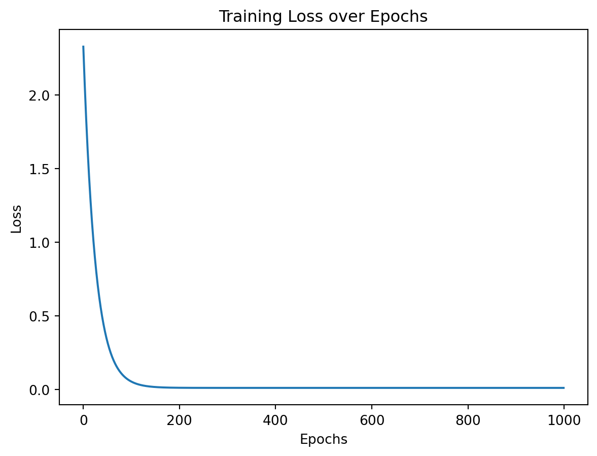
Create Linear Model via nn.Sequential

lr = 0.01
n_epochs = 1000
model = nn.Sequential(nn.Linear(1, 1)).to(device)
loss_fn = nn.MSELoss(reduction='mean')
optimizer = optim.SGD(model.parameters(), lr=lr)

losses = []
for t in range(n_epochs):
    model.train()
    # step 1: make prediction (forward pass)
    y_hat = model(x_tensor)
    # step 2: compute loss
    loss = loss_fn(y_tensor, y_hat)
    losses.append(loss.item())
    # step 3: clear old and compute current gradients
    optimizer.zero_grad() # clear old gradients
    loss.backward()       # compute current gradients
    # step 4: update parameters via an optimizer (e.g. SGD)
    optimizer.step() 

print(model.state_dict())
plt.plot(losses)
plt.xlabel('Epochs')
plt.ylabel('Loss')
plt.title('Training Loss over Epochs')
plt.show()

OrderedDict({'0.weight': tensor([[1.9959]]), '0.bias': tensor([1.0072])})

Dataset and Data Loader

from torch.utils.data import Dataset, TensorDataset
class myDataset(Dataset):
    def __init__(self, x, y):
        self.x = x_tensor
        self.y = y_tensor
    def __getitem__(self, index):
        return self.x[index], self.y[index]
    
    def __len__(self):
        return len(self.x)

train_data = myDataset(x_tensor, y_tensor)
print('Length of train_data:', len(train_data))
print('First item in train_data:', train_data[0])

train_data1 = TensorDataset(x_tensor, y_tensor)
print('Length of train_data1:', len(train_data1))
print('First item in train_data1:', train_data1[0])

Length of train_data: 1000
First item in train_data: (tensor([0.4967]), tensor([2.1334]))
Length of train_data1: 1000
First item in train_data1: (tensor([0.4967]), tensor([2.1334]))

Solve Linear Regression with Dataset and Data Loader

from torch.utils.data import DataLoader
train_loader = DataLoader(train_data, batch_size=50, shuffle=True)
lr = 0.01
n_epochs = 1000
model = nn.Sequential(nn.Linear(1, 1)).to(device)
loss_fn = nn.MSELoss(reduction='mean')
optimizer = optim.SGD(model.parameters(), lr=lr)
for t in range(n_epochs):
    for x_batch, y_batch in train_loader:
        x_batch = x_batch.to(device)
        y_batch = y_batch.to(device)
        model.train()
        # step 1: make prediction (forward pass)
        y_hat = model(x_batch)
        # step 2: compute loss
        loss = loss_fn(y_batch, y_hat)
        # step 3: clear old and compute current gradients
        optimizer.zero_grad() # clear old gradients
        loss.backward()       # compute current gradients
        # step 4: update parameters via an optimizer (e.g. SGD)
        optimizer.step()       
print(model.state_dict())

OrderedDict({'0.weight': tensor([[1.9958]]), '0.bias': tensor([1.0073])})

Evaluation in validation set

from torch.utils.data import random_split
dataset = TensorDataset(x_tensor, y_tensor)
train_dataset, val_dataset = random_split(dataset, [800, 200])
train_loader = DataLoader(train_dataset, batch_size=40)
val_loader = DataLoader(val_dataset, batch_size=20)
losses = []
val_losses = []

for t in range(n_epochs):
    for x_batch, y_batch in train_loader:
        x_batch = x_batch.to(device)
        y_batch = y_batch.to(device)

        model.train()
        # step 1: make prediction (forward pass)
        y_hat = model(x_batch)
        # step 2: compute loss
        loss = loss_fn(y_batch, y_hat)
        # step 3: clear old and compute current gradients
        optimizer.zero_grad() # clear old gradients
        loss.backward()       # compute current gradients
        # step 4: update parameters via an optimizer (e.g. SGD)
        optimizer.step() 
        
        # store the loss for plotting later
        losses.append(loss)
    
    # validation step (no need to track gradients)
    with torch.no_grad():
        for x_val, y_val in val_loader:
            model.eval()
            # step 1: prediction
            y_hat = model(x_val.to(device))
            # step 2: compute loss
            val_loss = loss_fn(y_val.to(device), y_hat)
            val_losses.append(val_loss.item())
print(model.state_dict())

OrderedDict({'0.weight': tensor([[1.9960]]), '0.bias': tensor([1.0072])})

Summary

No need to manually compute gradients; PyTorch’s autograd does it for you.
Use torch.nn for loss functions and optimizers.
Use nn.Sequential for building models in a modular way.
Use torch.utils.data.Dataset and DataLoader for data handling.
Use validation sets to evaluate model performance.
Reference