PyTorch: Logistic Regression

Logistic Regression Model

The logistic regression model estimates the probability of the label \(y\) given the input \(x\) by:

\[ \mathbb{P}(y = 1) = \sigma(w^\top x + b) \]

Here:

• \(x \in \mathbb{R}^d\) is the input vector, \(y \in \{0, 1\}\) is the binary label
  
• \(w \in \mathbb{R}^d\) is the weight vector, \(b \in \mathbb{R}\) is the bias (intercept)
  
• \(\sigma(z) = \dfrac{1}{1 + e^{-z}} = \dfrac{e^z}{1 + e^z}\) is the sigmoid function

---

Binary Cross-Entropy Loss

The loss function we minimize is the binary cross-entropy:

\[ L(w, b) = -\frac{1}{n} \sum_{i=1}^n \left[ y_i \log(\hat{y}_i) + (1 - y_i) \log(1 - \hat{y}_i) \right] \]

Here:

• \(n\) is the number of training examples
• \(y_i\) is the true label for the \(i\)-th sample
• \(\hat{y}_i = \sigma(w^\top x_i + b)\) is the predicted probability

Intuition

• If \(y_i = \hat{y}_i = 1\) for all \(i\), the loss is 0 — perfect prediction.
• If \(y_i = \hat{y}_i = 0\) for all \(i\), the loss is also 0.
• If \(y_i = 1\), \(\hat{y}_i = 0\), the loss becomes infinite — the worst-case prediction.

---

Deriving the Gradient

We start with the individual loss for each sample:

\[ L_i = -\left[ y_i \log(\sigma(z_i)) + (1 - y_i) \log(1 - \sigma(z_i)) \right], \]

where \(z_i = w^\top x_i + b\). Using the identity \(\frac{d\sigma(z)}{dz} = \sigma(z)(1 - \sigma(z))\), we obtain the gradient:

\[\begin{align*} \frac{\partial L_i}{\partial z_i} &= -\left[ y_i \frac{1}{\sigma(z_i)} \frac{\partial \sigma(z_i)}{\partial z_i} + (1 - y_i) \frac{-1}{1 - \sigma(z_i)} \frac{\partial \sigma(z_i)}{\partial z_i} \right]\\ &= -\left[ y_i \bigl(1 - \sigma(z_i)\bigr) - (1 - y_i) \sigma(z_i) \right]\\ &= \sigma(z_i) - y_i\\ &= \hat{y}_i - y_i. \end{align*}\]

By the chain rule, we can compute the gradient of the loss w.r.t. the weights \(w\) and bias \(b\): \[\begin{align*} \frac{\partial L_i}{\partial w} &= \frac{\partial L_i}{\partial z_i} \cdot \frac{\partial z_i}{\partial w} = (\hat y_i - y_i) x_i,\\ \frac{\partial L_i}{\partial b} &= \frac{\partial L_i}{\partial z_i} \cdot \frac{\partial z_i}{\partial b} = (\hat y_i - y_i). \end{align*}\]

Averaging over all \(n\) samples,the gradients become:

\[\begin{equation} \frac{\partial L}{\partial w} = \frac{1}{n} \sum_{i=1}^n (\hat{y}_i - y_i) x_i \quad \text{ and } \quad \frac{\partial L}{\partial b} = \frac{1}{n} \sum_{i=1}^n (\hat{y}_i - y_i). \end{equation}\]

---

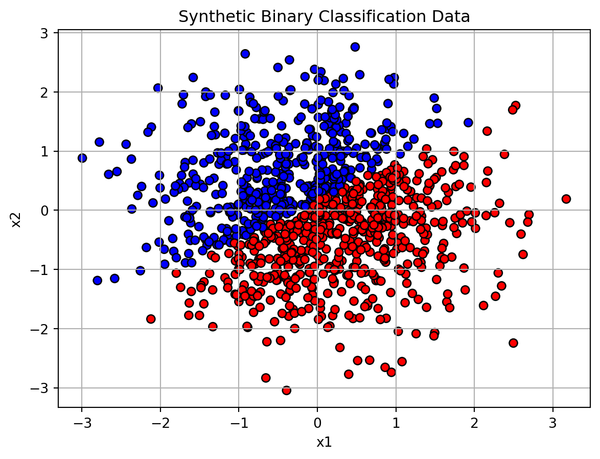
Step 1: Data Generation

import numpy as np
import matplotlib.pyplot as plt

np.random.seed(0)
n, d = 1000, 2
X = np.random.randn(n, d)
true_w = np.array([2.0, -3.0])
bias = 0.5

logits = X @ true_w + bias
probs = 1 / (1 + np.exp(-logits))
y = (probs > 0.5).astype(np.float32)

plt.scatter(X[:, 0], X[:, 1], c=y, cmap='bwr', edgecolor='k')
plt.title("Synthetic Binary Classification Data")
plt.xlabel("x1")
plt.ylabel("x2")
plt.grid(True)
plt.show()

---

Step 2: Logistic Regression with NumPy

def sigmoid(z):
    return 1 / (1 + np.exp(-z))

def binary_cross_entropy(y_true, y_pred):
    eps = 1e-7
    return -np.mean(y_true * np.log(y_pred + eps) + (1 - y_true) * np.log(1 - y_pred + eps))

w = np.zeros(2)
b = 0.0
lr = 0.1

for epoch in range(100):
    z = X @ w + b
    y_pred = sigmoid(z)
    loss = binary_cross_entropy(y, y_pred)

    dz = y_pred - y
    dw = X.T @ dz / n
    db = np.mean(dz)

    w -= lr * dw
    b -= lr * db

    if epoch % 10 == 0:
        print(f"Epoch {epoch}, Loss: {loss:.4f}")

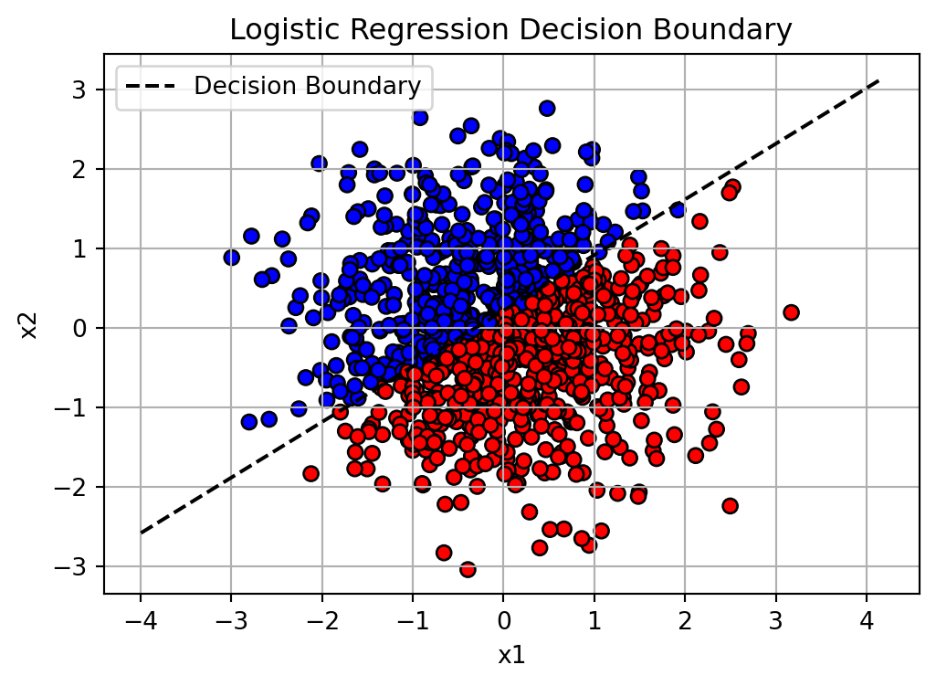
# Plotting the decision boundary
x_min, x_max = X[:, 0].min() - 1, X[:, 0].max() + 1
x_vals = np.linspace(x_min, x_max, 100)
# Solve for x2 on the decision boundary line: w1*x1 + w2*x2 + b = 0
# => x2 = -(w1*x1 + b)/w2
y_vals = -(w[0] * x_vals + b) / w[1]

# Plot
plt.figure(figsize=(6, 4))
plt.scatter(X[:, 0], X[:, 1], c=y, cmap='bwr', edgecolor='k')
plt.plot(x_vals, y_vals, 'k--', label='Decision Boundary')
plt.title("Logistic Regression Decision Boundary")
plt.xlabel("x1")
plt.ylabel("x2")
plt.legend()
plt.grid(True)
plt.show()

Epoch 0, Loss: 0.6931
Epoch 10, Loss: 0.5710
Epoch 20, Loss: 0.4932
Epoch 30, Loss: 0.4403
Epoch 40, Loss: 0.4019
Epoch 50, Loss: 0.3726
Epoch 60, Loss: 0.3495
Epoch 70, Loss: 0.3305
Epoch 80, Loss: 0.3147
Epoch 90, Loss: 0.3013

---

Step 3: Logistic Regression with PyTorch

import torch
from torch import nn

X_tensor = torch.tensor(X, dtype=torch.float32)
y_tensor = torch.tensor(y, dtype=torch.float32).view(-1, 1)

model = nn.Sequential(
    nn.Linear(d, 1),
    nn.Sigmoid()
)

loss_fn = nn.BCELoss()
optimizer = torch.optim.SGD(model.parameters(), lr=0.1)

for epoch in range(100):
    model.train()  # set model to training mode
    # step 1: make prediction (forward pass)
    y_pred = model(X_tensor)
    # step 2: compute loss
    loss = loss_fn(y_pred, y_tensor)
    # step 3: clear old and compute current gradients
    optimizer.zero_grad() # clear old gradients
    loss.backward()       # compute current gradients
    # step 4: update parameters
    optimizer.step()

    if epoch % 10 == 0:
        print(f"Epoch {epoch}, Loss: {loss.item():.4f}")

Epoch 0, Loss: 0.6921
Epoch 10, Loss: 0.5684
Epoch 20, Loss: 0.4893
Epoch 30, Loss: 0.4356
Epoch 40, Loss: 0.3970
Epoch 50, Loss: 0.3678
Epoch 60, Loss: 0.3449
Epoch 70, Loss: 0.3263
Epoch 80, Loss: 0.3108
Epoch 90, Loss: 0.2977